Optimizing Your First Strategy

So, you’ve finally created your first strategy, but it’s not as profitable as you had hoped? Or maybe you already have a profitable strategy, but are wondering whether or not you could improve its performance even more? Or perhaps you are trying to tweak other aspects of your strategy, such as entry / exit points, but can’t be bothered to fine-tune parameters for hours on end?

These are the problems that Naxbot’s integrated optimizer aims to solve. By leveraging a metaheuristic optimization algorithm, Naxbot is capable of finding optimum parameters for any strategy you throw at it.

In this tutorial, we will be optimizing the strategy created in “Create Your First Strategy”, but you are free to follow along with any strategy you may already have.

Strategy Preparation

First, we will need to prepare our strategy script to allow the optimizer to change some of its parameters. As a reminder, we are working with the following strategy:


function process()
    local fast_length = 5
    local slow_length = 17
 
    local fast_rsi = rsi(close, fast_length)
    local slow_rsi = rsi(close, slow_length)
 
    local divergence = fast_rsi - slow_rsi
 
    local long_entry_condition = crossover(divergence, 0)
    local short_entry_condition = crossunder(divergence, 0)
 
    -- we declare a variable to avoid
    -- multiple future calculations
    local distance = atr(21)
 
    -- we now calculate both long & short stop loss,
    -- and then later decide which one to use based
    -- on whether the signal is long or not.
    local stop_loss_distance = distance * 1.5
    local long_stop_loss = close - stop_loss_distance
    local short_stop_loss = close + stop_loss_distance
    local stop_loss = lif(long_entry_condition, long_stop_loss, short_stop_loss)
 
    -- we do the same for our take profit target
    local tp_1_distance = distance * 3
    local long_tp_1 = close + tp_1_distance
    local short_tp_1 = close - tp_1_distance
    local tp_1 = lif(long_entry_condition, long_tp_1, short_tp_1)
 
    return {
        long_entry_condition = long_entry_condition,
        short_entry_condition = short_entry_condition,
        long_exit_condition = constant(false),
        short_exit_condition = constant(false),
        stop_loss = stop_loss,
        tp_1 = tp_1,
        fast_rsi = fast_rsi,
        slow_rsi = slow_rsi,
        divergence = divergence,
    }
end

In our “Create Your First Strategy” tutorial, this particular strategy was actually not profitable, so let’s see if the optimizer can turn it into a profitable one. First, we’ll need to define which parameters we want the optimizer to change. In this case, the two RSI lengths seem like fine candidates. We’ll change the process function to take in actual parameters, and use the current lengths as default values:


function process(fast_length, slow_length)
~   local fast_length = fast_length or 5
~   local slow_length = slow_length or 17
 
    local fast_rsi = rsi(close, fast_length)
    local slow_rsi = rsi(close, slow_length)
 
    local divergence = fast_rsi - slow_rsi
 
    local long_entry_condition = crossover(divergence, 0)
    local short_entry_condition = crossunder(divergence, 0)
 
    -- we declare a variable to avoid
    -- multiple future calculations
    local distance = atr(21)
 
    -- we now calculate both long & short stop loss,
    -- and then later decide which one to use based
    -- on whether the signal is long or not.
    local stop_loss_distance = distance * 1.5
    local long_stop_loss = close - stop_loss_distance
    local short_stop_loss = close + stop_loss_distance
    local stop_loss = lif(long_entry_condition, long_stop_loss, short_stop_loss)
 
    -- we do the same for our take profit target
    local tp_1_distance = distance * 3
    local long_tp_1 = close + tp_1_distance
    local short_tp_1 = close - tp_1_distance
    local tp_1 = lif(long_entry_condition, long_tp_1, short_tp_1)
 
    return {
        long_entry_condition = long_entry_condition,
        short_entry_condition = short_entry_condition,
        long_exit_condition = constant(false),
        short_exit_condition = constant(false),
        stop_loss = stop_loss,
        tp_1 = tp_1,
        fast_rsi = fast_rsi,
        slow_rsi = slow_rsi,
        divergence = divergence,
    }
end

And that’s all it takes to prepare a strategy for the optimizer. Painless, wasn’t it? Next, we’ll set up the optimizer job.

Optimizer Panel

Oh no, it looks like the inside of a space ship!

Not to worry! While all these settings may seem confusing at first, things are actually quite simple once you break them down.

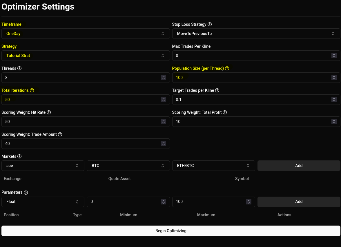
First, let’s begin by selecting the strategy we want to optimize (you did save your strategy, right?). Then, we can go ahead and tune down both the total iterations and the population size per thread, since we are only optimizing two parameters that can’t have all that many values. We’ll also change the timeframe to OneDay, since that’s the timeframe we backtested with earlier.

Note

If your CPU has fewer than 8 cores, you may also need to tune down the Threads parameter.

When you’re done, your view should look something like this:

Optimizer Settings

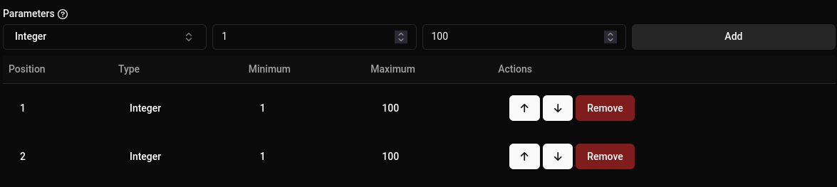
Next, we’ll need to tell the optimizer about the parameters we want it to, well, optimize. In our case, fast_length and slow_length are both integers, so down at the Parameters section, we’ll select Integer. As for possible values, we’ll just pick a minimum of 1 and a maximum of 100 (arbitrarily chosen)`. Add two of the same parameter type, so it looks like this:

Optimizer Parameters

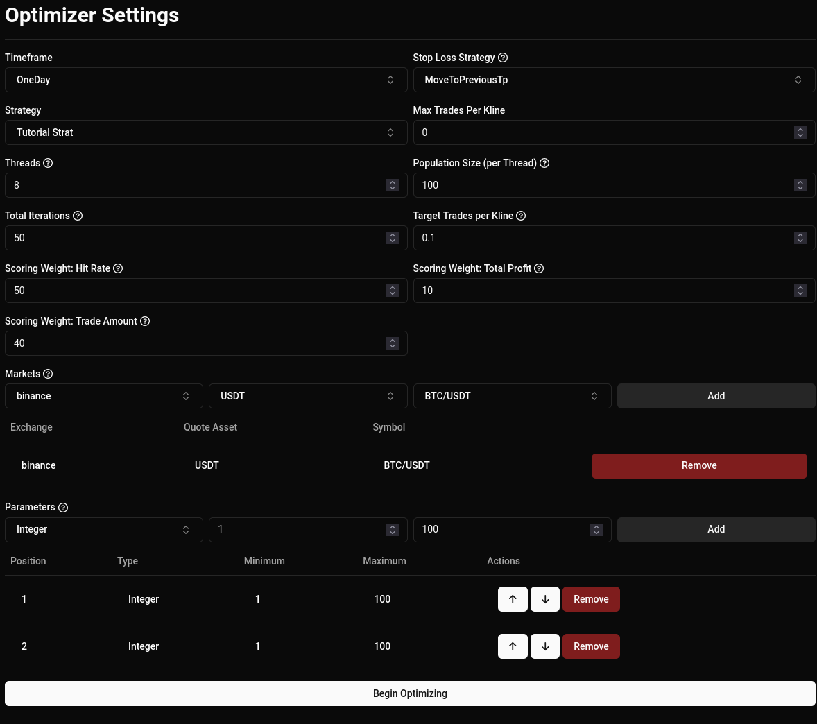
Lastly, we need to tell it which markets we want to optimize the strategy on. For simplicity’s sake, we’ll also go with binance and ETH/USDT like we did when we created the strategy, but note that in reality, you will want to avoid optimizing on the same markets you backtest and/or plan to actively trade, due to potential issues with overfitting.

The final settings should look similar to this:

Optimizer Settings

All that’s left now is to hit “Begin Optimizing” and watch the optimizer do its magic!

Once the optimizer is done, the results will be presented to you at the top of the page:

Optimizer Results

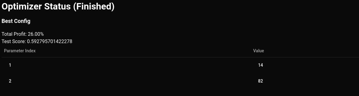
So far so good, now let’s plop these numbers back into our strategy and run another backtest on binance and BTC/USDT:


function process(fast_length, slow_length)
    local fast_length = fast_length or 14
    local slow_length = slow_length or 82
 
    local fast_rsi = rsi(close, fast_length)
    local slow_rsi = rsi(close, slow_length)
 
    local divergence = fast_rsi - slow_rsi
 
    local long_entry_condition = crossover(divergence, 0)
    local short_entry_condition = crossunder(divergence, 0)
 
    -- we declare a variable to avoid
    -- multiple future calculations
    local distance = atr(21)
 
    -- we now calculate both long & short stop loss,
    -- and then later decide which one to use based
    -- on whether the signal is long or not.
    local stop_loss_distance = distance * 1.5
    local long_stop_loss = close - stop_loss_distance
    local short_stop_loss = close + stop_loss_distance
    local stop_loss = lif(long_entry_condition, long_stop_loss, short_stop_loss)
 
    -- we do the same for our take profit target
    local tp_1_distance = distance * 3
    local long_tp_1 = close + tp_1_distance
    local short_tp_1 = close - tp_1_distance
    local tp_1 = lif(long_entry_condition, long_tp_1, short_tp_1)
 
    return {
        long_entry_condition = long_entry_condition,
        short_entry_condition = short_entry_condition,
        long_exit_condition = constant(false),
        short_exit_condition = constant(false),
        stop_loss = stop_loss,
        tp_1 = tp_1,
        fast_rsi = fast_rsi,
        slow_rsi = slow_rsi,
        divergence = divergence,
    }
end

The backtest results are as follows:

Backtest results

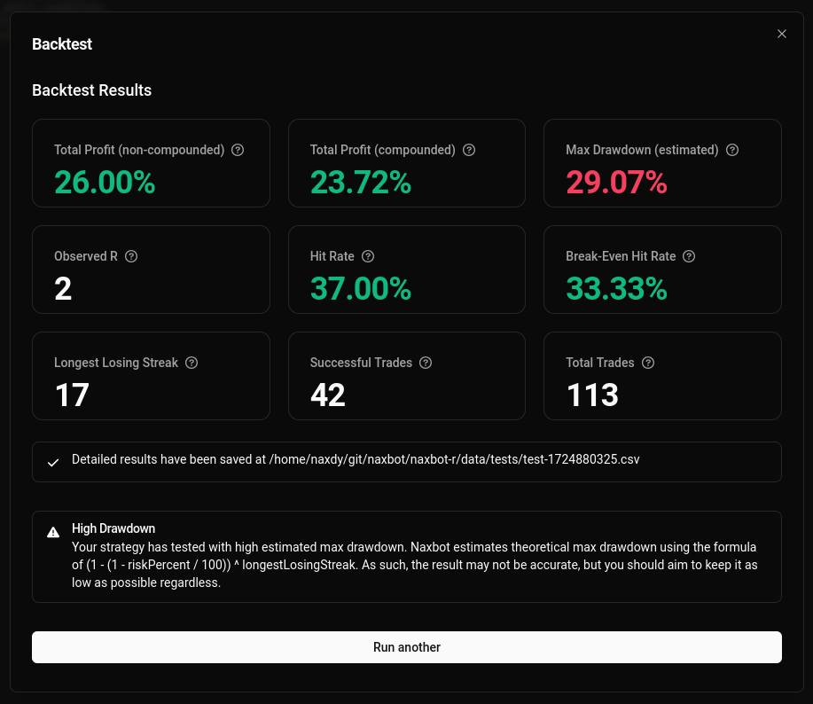
This is already much better than what we previously had, but the profit still isn’t too overwhelming. Perhaps there is a way to optimize this even more…

Further Optimization

Now that we know how to operate the optimizer, we can take things to the next level. In the previous section, we used the optimizer to optimize the lengths of both of our RSI indicators. But what if we used it to optimize stop loss & take profit targets?

Well, we can do that too, of course! We simply add two new parameters to the function and use those parameters in our take profit & stop loss calculations. The resulting script will look a little like this:


function process(fast_length, slow_length, stop_loss_multiplier, tp_1_multiplier)
    local fast_length = fast_length or 14
    local slow_length = slow_length or 82
+   stop_loss_multiplier = stop_loss_multiplier or 1.5
+   tp_1_multiplier = tp_1_multiplier or 3
 
    local fast_rsi = rsi(close, fast_length)
    local slow_rsi = rsi(close, slow_length)
 
    local divergence = fast_rsi - slow_rsi
 
    local long_entry_condition = crossover(divergence, 0)
    local short_entry_condition = crossunder(divergence, 0)
 
    -- we declare a variable to avoid
    -- multiple future calculations
    local distance = atr(21)
 
    -- we now calculate both long & short stop loss,
    -- and then later decide which one to use based
    -- on whether the signal is long or not.
~   local stop_loss_distance = distance * stop_loss_multiplier
    local long_stop_loss = close - stop_loss_distance
    local short_stop_loss = close + stop_loss_distance
    local stop_loss = lif(long_entry_condition, long_stop_loss, short_stop_loss)
 
    -- we do the same for our take profit target
~   local tp_1_distance = distance * tp_1_multiplier
    local long_tp_1 = close + tp_1_distance
    local short_tp_1 = close - tp_1_distance
    local tp_1 = lif(long_entry_condition, long_tp_1, short_tp_1)
 
    return {
        long_entry_condition = long_entry_condition,
        short_entry_condition = short_entry_condition,
        long_exit_condition = constant(false),
        short_exit_condition = constant(false),
        stop_loss = stop_loss,
        tp_1 = tp_1,
        fast_rsi = fast_rsi,
        slow_rsi = slow_rsi,
        divergence = divergence,
    }
end

We’ll set up the optimizer job the same, but this time we’ll add two float parameters at the end, for our multipliers:

Optimizer Settings

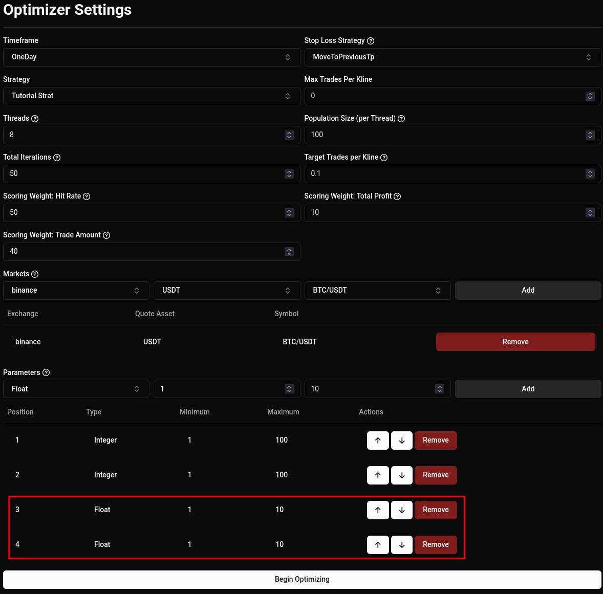
Let’s optimize and have a look at the results!

Optimizer Results

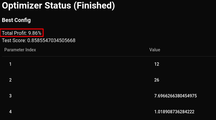
That’s strange, the configuration suggested by the optimizer is generating less profit than the previous one. But why? Let’s perform a backtest and have a look at the results in more detail:

Backtest Results

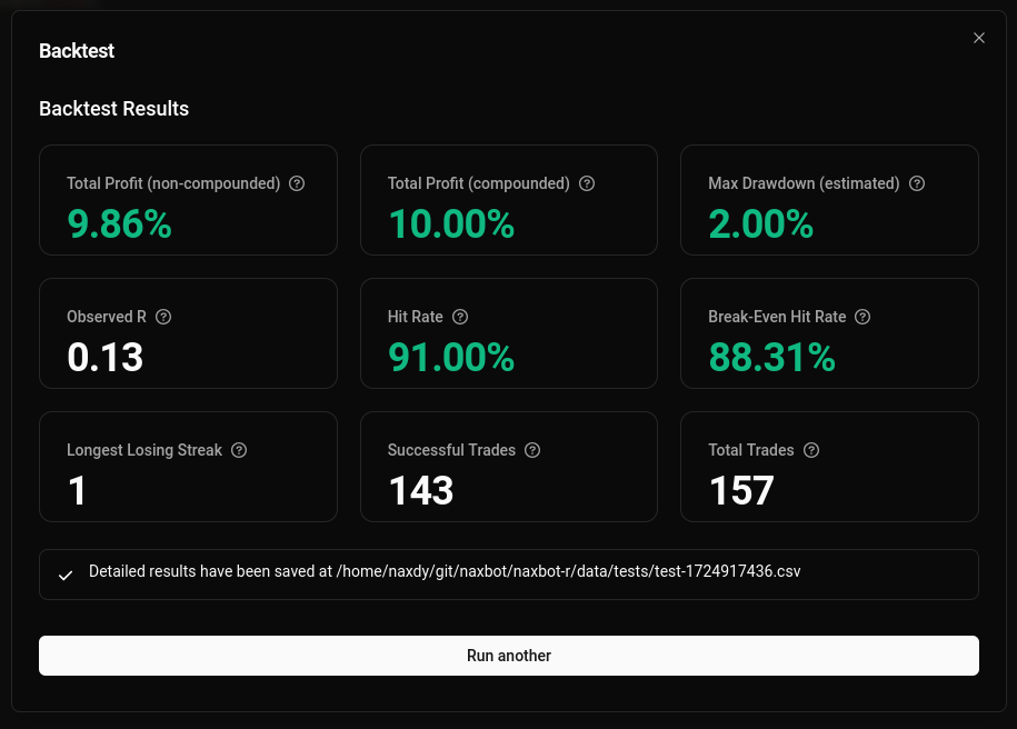
So, while the total profit has decreased, both the hit-rate and the break-even hit rate have skyrocketed.

To understand this, it is important to understand how the optimizer picks its configuration. You see, when it comes to evaluating trading strategies, there isn’t a single end-all-be-all metric that can be used to rank them. Instead, what’s important is usually a combination of hit rate, overall profitability, risk-reward ratio, and trade frequency.

Naxbot’s optimizer takes all of these into account, but the weight at which these are evaluated is defined by the user. In fact, that’s the reason why the optimizer has picked a config with a fairly high hit rate of 91%, but a lacking overall profit.

Weight Adjustment

To mitigate this, all we need to do is to tell the optimizer that we care more about profit, than we do about hit rate. Let’s change the scoring weights so that the total profit weight is greater than the hit rate weight:

Optimizer Settings

💡

Tip

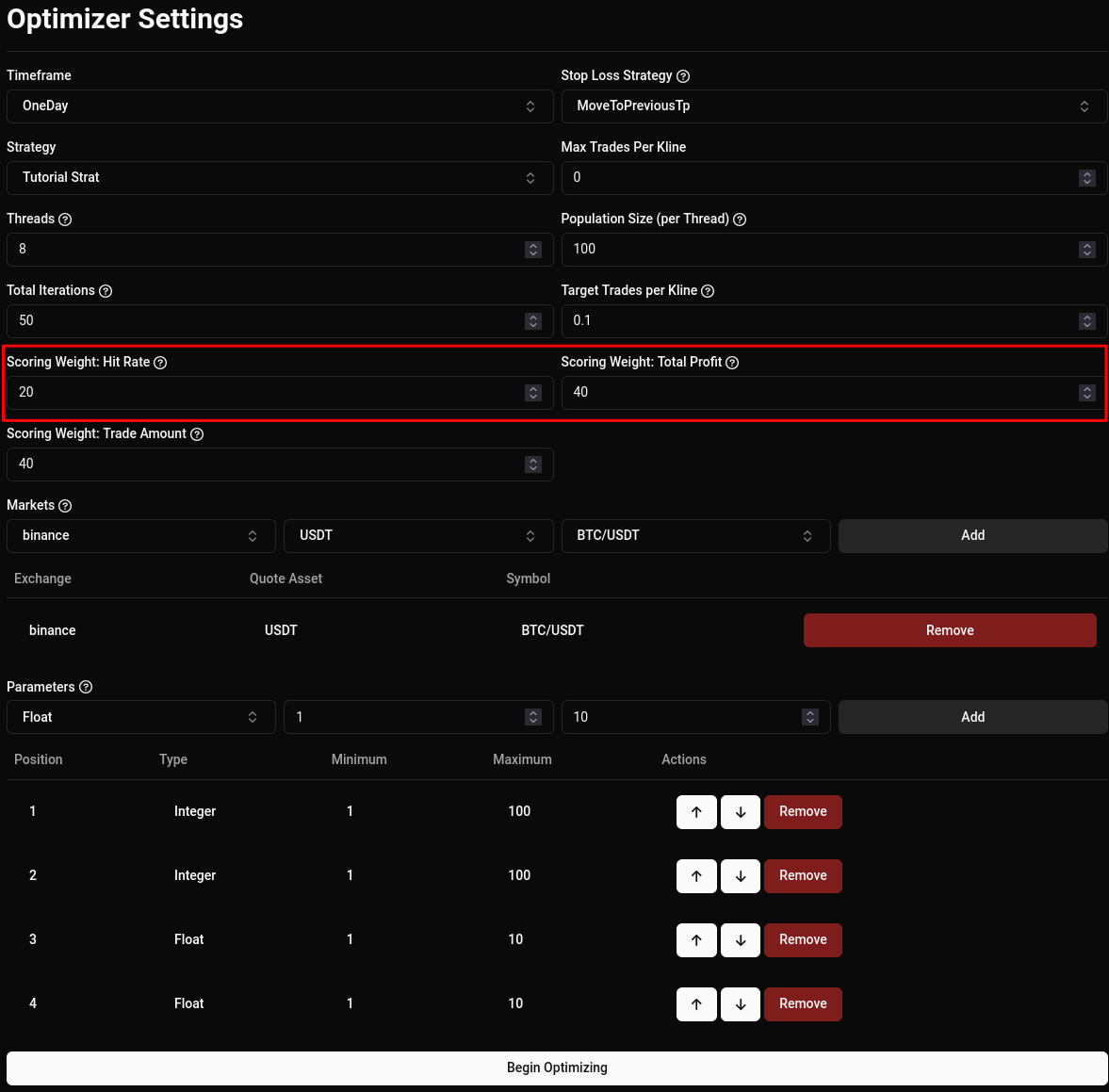
At this stage, it is also a good idea to increase total iterations, population size per thread, and thread count (if you can), since the parameters we are optimizing for are more complex than the ones we optimized for in the initial example.

Finally, let’s have a look at the result:

Optimizer Results

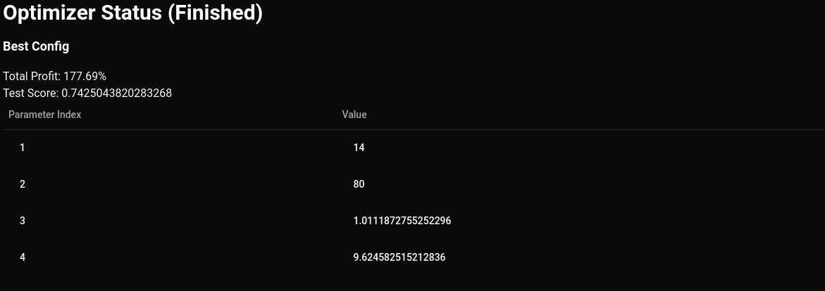
This already looks much more promising. Let’s pop these final values into our strategy, so we can perform a backtest:


function process(fast_length, slow_length, stop_loss_multiplier, tp_1_multiplier)
    local fast_length = fast_length or 14
    local slow_length = slow_length or 80
    stop_loss_multiplier = stop_loss_multiplier or 1.0111872755252296
    tp_1_multiplier = tp_1_multiplier or 9.624582515212836
 
    local fast_rsi = rsi(close, fast_length)
    local slow_rsi = rsi(close, slow_length)
 
    local divergence = fast_rsi - slow_rsi
 
    local long_entry_condition = crossover(divergence, 0)
    local short_entry_condition = crossunder(divergence, 0)
 
    -- we declare a variable to avoid
    -- multiple future calculations
    local distance = atr(21)
 
    -- we now calculate both long & short stop loss,
    -- and then later decide which one to use based
    -- on whether the signal is long or not.
    local stop_loss_distance = distance * stop_loss_multiplier
    local long_stop_loss = close - stop_loss_distance
    local short_stop_loss = close + stop_loss_distance
    local stop_loss = lif(long_entry_condition, long_stop_loss, short_stop_loss)
 
    -- we do the same for our take profit target
    local tp_1_distance = distance * tp_1_multiplier
    local long_tp_1 = close + tp_1_distance
    local short_tp_1 = close - tp_1_distance
    local tp_1 = lif(long_entry_condition, long_tp_1, short_tp_1)
 
    return {
        long_entry_condition = long_entry_condition,
        short_entry_condition = short_entry_condition,
        long_exit_condition = constant(false),
        short_exit_condition = constant(false),
        stop_loss = stop_loss,
        tp_1 = tp_1,
        fast_rsi = fast_rsi,
        slow_rsi = slow_rsi,
        divergence = divergence,
    }
end

Performing a backtest on binance and BTC/USDT yields the following result:

Backtest Results

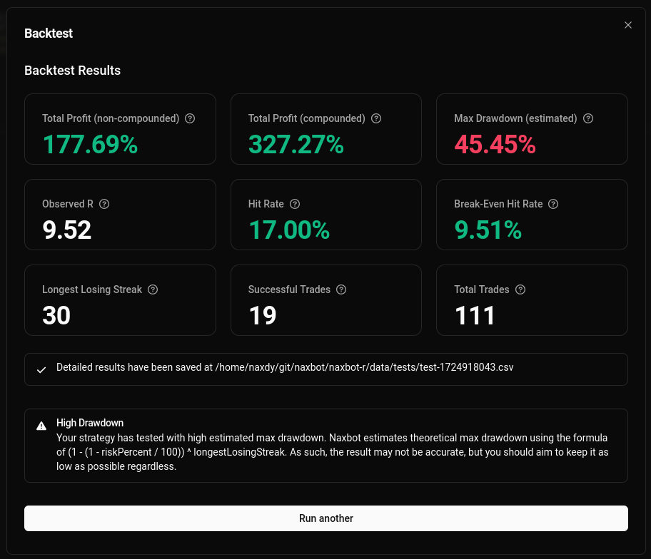
These results are much better than what we started with. However, there are still a few problems with this configuration, mainly the longest losing streak and the resulting max drawdown. As it stands, you need some pretty big cojones to be trading this strategy. This can be adjusted by limiting the range of the stop loss & tp target parameters the optimizer may pick from, or by adjusting the hit rate vs. total profit scoring weights, like we did before.

Considering we started with a very simple strategy however, these results are pretty phenomenal. You can imagine the kind of results you can achieve with something more sophisticated.

Now you know how to optimize your strategy with Naxbot. If you have any further questions, don’t hesitate to ask in the proper forums!