Create Your First Strategy

Creating your first strategy may seem like a daunting task, especially if you have little to no programming experience. However, Lua is extremely beginner friendly, and Naxbot’s ecosystem has been built to enable even novice programmers to create their own strategies with ease.

Where to begin

The first question you will need to ask yourself is what kind of strategy you want to implement. Do you want to create a trend-following strategy, or do you want to trade reversals? Do you want to make long-term trades, or focus on short-term scalping?

A good starting point for finding some strategies is TradingView , which you can also search for popular indicators. If you want to learn how to transcribe indicators & strategies from TradingView to Naxbot, have a look at our guide for transcribing TradingView strategies.

For this tutorial however, we will be using a simple strategy based on the relative strength index (RSI).

Defining the Strategy

As mentioned before, we will be using a simple RSI based strategy. Specifically, we will be calculating the difference between a faster moving RSI and a slower one, and using that difference to get our long & short signals.

Let’s begin by heading over to the Strategy tab in the Naxbot web interface. Go ahead and remove the default strategy, and replace it with the following “skeleton” strategy:


function process()
    return {
        long_entry_condition = constant(false),
        short_entry_condition = constant(false),
        long_exit_condition = constant(false),
        short_exit_condition = constant(false),
        stop_loss = constant(0),
        tp_1 = constant(0),
    }
end

This will leave us with a clean slate to work with. So far so good, but our strategy doesn’t do anything right now. Let’s start by implementing the two RSI indicators we talked about earlier:


function process()
+   local fast_length = 5
+   local slow_length = 17
 
+   local fast_rsi = rsi(close, fast_length)
+   local slow_rsi = rsi(close, slow_length)
 
    return {
        long_entry_condition = constant(false),
        short_entry_condition = constant(false),
        long_exit_condition = constant(false),
        short_exit_condition = constant(false),
        stop_loss = constant(0),
        tp_1 = constant(0),
    }
end

Now we’re getting somewhere. We can add the two indicators to our return table, so we can plot them into a spreadsheet, just to get an idea of what it looks like:


function process()
    local fast_length = 5
    local slow_length = 17
 
    local fast_rsi = rsi(close, fast_length)
    local slow_rsi = rsi(close, slow_length)
 
    return {
        long_entry_condition = constant(false),
        short_entry_condition = constant(false),
        long_exit_condition = constant(false),
        short_exit_condition = constant(false),
        stop_loss = constant(0),
        tp_1 = constant(0),
+       fast_rsi = fast_rsi,
+       slow_rsi = slow_rsi,
    }
end

💡

Tip

To plot a strategy, click on the “Plot” button in the top right, pick your target market & timeframe of choice, and then click on “Download Plot”.

Plot UI

Next, let’s subtract the slow RSI from the fast RSI to get our divergence. We’ll also add it to the return table, so we can plot it:


function process()
    local fast_length = 5
    local slow_length = 17
 
    local fast_rsi = rsi(close, fast_length)
    local slow_rsi = rsi(close, slow_length)
 
+   local divergence = fast_rsi - slow_rsi
 
    return {
        long_entry_condition = constant(false),
        short_entry_condition = constant(false),
        long_exit_condition = constant(false),
        short_exit_condition = constant(false),
        stop_loss = constant(0),
        tp_1 = constant(0),
        fast_rsi = fast_rsi,
        slow_rsi = slow_rsi,
+       divergence = divergence,
    }
end

Now we need to define our long & short entry conditions. Since the RSI is an oscillating indicator (meaning it is moving around a fixed point, in this case the number 0), we can simply define our entry conditions as crossover / crossunder in relation to the fixed point it is oscillating around. Luckily, Naxbot provides some handy functions to do just that:


function process()
    local fast_length = 5
    local slow_length = 17
 
    local fast_rsi = rsi(close, fast_length)
    local slow_rsi = rsi(close, slow_length)
 
    local divergence = fast_rsi - slow_rsi
 
+   local long_entry_condition = crossover(divergence, 0)
+   local short_entry_condition = crossunder(divergence, 0)
 
    return {
~       long_entry_condition = long_entry_condition,
~       short_entry_condition = short_entry_condition,
        long_exit_condition = constant(false),
        short_exit_condition = constant(false),
        stop_loss = constant(0),
        tp_1 = constant(0),
        fast_rsi = fast_rsi,
        slow_rsi = slow_rsi,
        divergence = divergence,
    }
end

Things are finally starting to shape up! The only things we’re missing now is a stop loss and a take profit target. For this example, we’ll use multiples of the average true range to get our stop loss & take profit targets, but you can use any indicator you like:


function process()
    local fast_length = 5
    local slow_length = 17
 
    local fast_rsi = rsi(close, fast_length)
    local slow_rsi = rsi(close, slow_length)
 
    local divergence = fast_rsi - slow_rsi
 
    local long_entry_condition = crossover(divergence, 0)
    local short_entry_condition = crossunder(divergence, 0)
 
+   -- we declare a variable to avoid
+   -- multiple future calculations
+   local distance = atr(21)
 
+   -- we set stop loss at 1.5x atr
+   local stop_loss = close - distance * 1.5
 
+   -- while setting tp_1 at 3x atr
+   local tp_1 = close + distance * 3
 
    return {
        long_entry_condition = long_entry_condition,
        short_entry_condition = short_entry_condition,
        long_exit_condition = constant(false),
        short_exit_condition = constant(false),
~       stop_loss = stop_loss,
~       tp_1 = tp_1,
        fast_rsi = fast_rsi,
        slow_rsi = slow_rsi,
        divergence = divergence,
    }
end

Perfect! Except for one thing: These stop loss and take profit targets are only valid for long trades. For short trades, our stop loss needs to be above our entry price, not below. We can fix this however, by using the lif function. Refer to our API Reference for more info on how it works. Here’s the final script:


function process()
    local fast_length = 5
    local slow_length = 17
 
    local fast_rsi = rsi(close, fast_length)
    local slow_rsi = rsi(close, slow_length)
 
    local divergence = fast_rsi - slow_rsi
 
    local long_entry_condition = crossover(divergence, 0)
    local short_entry_condition = crossunder(divergence, 0)
 
    -- we declare a variable to avoid
    -- multiple future calculations
    local distance = atr(21)
 
    -- we now calculate both long & short stop loss,
    -- and then later decide which one to use based
    -- on whether the signal is long or not.
    local stop_loss_distance = distance * 1.5
    local long_stop_loss = close - stop_loss_distance
    local short_stop_loss = close + stop_loss_distance
    local stop_loss = lif(long_entry_condition, long_stop_loss, short_stop_loss)
 
    -- we do the same for our take profit target
    local tp_1_distance = distance * 3
    local long_tp_1 = close + tp_1_distance
    local short_tp_1 = close - tp_1_distance
    local tp_1 = lif(long_entry_condition, long_tp_1, short_tp_1)
 
    return {
        long_entry_condition = long_entry_condition,
        short_entry_condition = short_entry_condition,
        long_exit_condition = constant(false),
        short_exit_condition = constant(false),
        stop_loss = stop_loss,
        tp_1 = tp_1,
        fast_rsi = fast_rsi,
        slow_rsi = slow_rsi,
        divergence = divergence,
    }
end

Awesome! Now, let’s backtest our new strategy. We’ll hit the backtest button in the top right, and select binance as our exchange, and BTC/USDT as our trading pair. Don’t forget to add a TP target too! The settings should look something like this:

Backtest example

Note

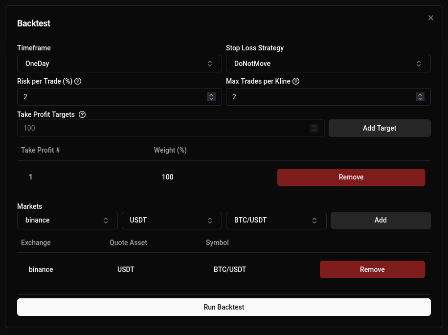
Since we only have 1 TP target, “Stop Loss Strategy” doesn’t come into play here.

Now, let’s see how our strategy performs!

Backtest result

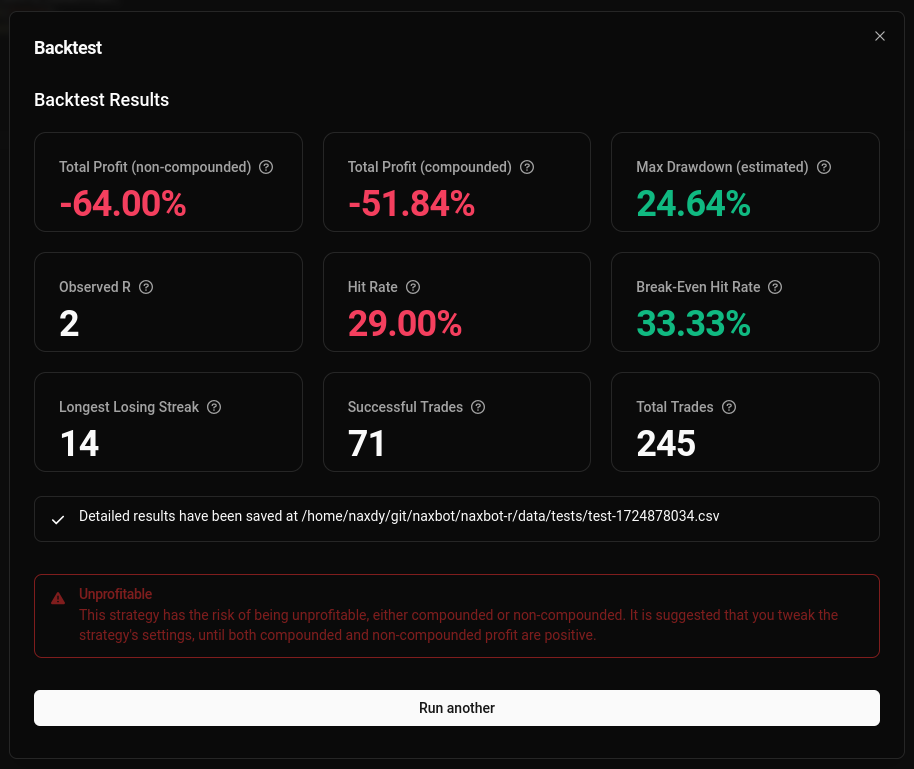
Well, now this isn’t too encouraging… But regardless, you have successfully created your first strategy!

And all hope is not yet lost, for Naxbot has an integrated optimizer that you can leverage in order to improve your strategy’s performance. Continue this tutorial in: Optimizing Your First Strategy to see if we can make this strategy profitable!

Create Your First Strategy

Where to begin

Defining the Strategy​

Defining the Strategy